N-Mass Pendulum
The pendulum system can be represented by a second order system of differential equations. To find the equations that guides this motion, we first need the Lagrangian. \[\mathcal{L}=T-U\] The second order component (angular acceleration) of the nth mass is guaranteed to be linear. It is given by: \[\frac{\mathrm{d}}{\mathrm{d}t}(\frac{\partial \mathcal{L}}{\partial \dot{\theta_n}}) - \frac{\partial \mathcal{L}}{\partial \theta_n} = 0\]
The x and y coordinates of the first mass (closest to the base) is given by: \[x = L_{1} \sin{\left(\theta_{1}{\left(t \right)} \right)}\] \[y = - L_{1} \cos{\left(\theta_{1}{\left(t \right)} \right)}\] In general the coordinates of the ith mass are... \[x_i = x_{i-1} + L_{1} \sin{\left(\theta_{i}{\left(t \right)} \right)}\] \[y_i = y_{i-1} - L_{1} \cos{\left(\theta_{i}{\left(t \right)} \right)}\] The kinetic and potential energy can be obtained by: \[T = \sum_{i=1}^n \frac{1}{2} m_i (x_i^2 + y_i^2)\] \[U = \sum_{i=1}^n m_i g y_i\] For example, the 3 mass system:
\[\mathcal{L} = 0.5 L_{1}^{2} m_{1} \left(\frac{d}{d t} \theta_{1}{\left(t \right)}\right)^{2} + L_{1} g m_{1}
\cos{\left(\theta_{1}{\left(t \right)} \right)} + g m_{2} \left(L_{1} \cos{\left(\theta_{1}{\left(t \right)}
\right)} + L_{2} \cos{\left(\theta_{2}{\left(t \right)} \right)}\right) + g m_{3} \left(L_{1}
\cos{\left(\theta_{1}{\left(t \right)} \right)} + L_{2} \cos{\left(\theta_{2}{\left(t \right)} \right)} + L_{3}
\cos{\left(\theta_{3}{\left(t \right)} \right)}\right) + 0.5 m_{2} \left(L_{1}^{2} \left(\frac{d}{d t}
\theta_{1}{\left(t \right)}\right)^{2} + 2 L_{1} L_{2} \cos{\left(\theta_{1}{\left(t \right)} -
\theta_{2}{\left(t \right)} \right)} \frac{d}{d t} \theta_{1}{\left(t \right)} \frac{d}{d t} \theta_{2}{\left(t
\right)} + L_{2}^{2} \left(\frac{d}{d t} \theta_{2}{\left(t \right)}\right)^{2}\right) + 0.5 m_{3}
\left(L_{1}^{2} \left(\frac{d}{d t} \theta_{1}{\left(t \right)}\right)^{2} + 2 L_{1} L_{2}
\cos{\left(\theta_{1}{\left(t \right)} - \theta_{2}{\left(t \right)} \right)} \frac{d}{d t} \theta_{1}{\left(t
\right)} \frac{d}{d t} \theta_{2}{\left(t \right)} + 2 L_{1} L_{3} \cos{\left(\theta_{1}{\left(t \right)} -
\theta_{3}{\left(t \right)} \right)} \frac{d}{d t} \theta_{1}{\left(t \right)} \frac{d}{d t} \theta_{3}{\left(t
\right)} + L_{2}^{2} \left(\frac{d}{d t} \theta_{2}{\left(t \right)}\right)^{2} + 2 L_{2} L_{3}
\cos{\left(\theta_{2}{\left(t \right)} - \theta_{3}{\left(t \right)} \right)} \frac{d}{d t} \theta_{2}{\left(t
\right)} \frac{d}{d t} \theta_{3}{\left(t \right)} + L_{3}^{2} \left(\frac{d}{d t} \theta_{3}{\left(t
\right)}\right)^{2}\right)\]
\[\mathcal{L} = 0.5 L_{1}^{2} m_{1} \left(\frac{d}{d t} \theta_{1}{\left(t \right)}\right)^{2} + L_{1} g m_{1}
\cos{\left(\theta_{1}{\left(t \right)} \right)}\]
\[+ g m_{2} \left(L_{1} \cos{\left(\theta_{1}{\left(t \right)}
\right)} + L_{2} \cos{\left(\theta_{2}{\left(t \right)} \right)}\right)\]
\[+ g m_{3} \left(L_{1}
\cos{\left(\theta_{1}{\left(t \right)} \right)} + L_{2} \cos{\left(\theta_{2}{\left(t \right)} \right)} + L_{3}
\cos{\left(\theta_{3}{\left(t \right)} \right)}\right)\]
\[+ 0.5 m_{2} \left(L_{1}^{2} \left(\frac{d}{d t}
\theta_{1}{\left(t \right)}\right)^{2} + 2 L_{1} L_{2} \cos{\left(\theta_{1}{\left(t \right)} -
\theta_{2}{\left(t \right)} \right)} \frac{d}{d t} \theta_{1}{\left(t \right)} \frac{d}{d t} \theta_{2}{\left(t
\right)}\right)\]
\[+ L_{2}^{2} \left(\frac{d}{d t} \theta_{2}{\left(t \right)}\right)^{2} + 0.5 m_{3}
\left(L_{1}^{2} \left(\frac{d}{d t} \theta_{1}{\left(t \right)}\right)^{2}\right)\]
\[+ 2 L_{1} L_{2}
\cos{\left(\theta_{1}{\left(t \right)} - \theta_{2}{\left(t \right)} \right)} \frac{d}{d t} \theta_{1}{\left(t
\right)} \frac{d}{d t} \theta_{2}{\left(t \right)}\]
\[+ 2 L_{1} L_{3} \cos{\left(\theta_{1}{\left(t \right)} -
\theta_{3}{\left(t \right)} \right)} \frac{d}{d t} \theta_{1}{\left(t \right)} \frac{d}{d t} \theta_{3}{\left(t
\right)}\]
\[+ L_{2}^{2} \left(\frac{d}{d t} \theta_{2}{\left(t \right)}\right)^{2} + 2 L_{2} L_{3}
\cos{\left(\theta_{2}{\left(t \right)} - \theta_{3}{\left(t \right)} \right)} \frac{d}{d t} \theta_{2}{\left(t
\right)} \frac{d}{d t} \theta_{3}{\left(t \right)}\]
\[+ L_{3}^{2} \left(\frac{d}{d t} \theta_{3}{\left(t
\right)}\right)^{2}\]
The equations can be quite massive, but they will be linear in terms of angular acceleration. We
can treat the Lagrangian equations of motion as a set of linear equations to solve for each
\(\ddot{\theta_n}\).
\[\begin{bmatrix}\ \ddot{\theta_1} \\ \ddot{\theta_2} \\ \ddot{\theta_3} \\ ... \\ \ddot{\theta_n} \end{bmatrix}
= \begin{bmatrix}\
f(\theta_1, \dot{\theta_1}, \theta_2, \dot{\theta_2}, \theta_3, \dot{\theta_3} ... , \theta_n, \dot{\theta_n})
\\
f(\theta_1, \dot{\theta_1}, \theta_2, \dot{\theta_2}, \theta_3, \dot{\theta_3} ... , \theta_n, \dot{\theta_n})
\\
f(\theta_1, \dot{\theta_1}, \theta_2, \dot{\theta_2}, \theta_3, \dot{\theta_3} ... , \theta_n, \dot{\theta_n})
\\
... \\
f(\theta_1, \dot{\theta_1}, \theta_2, \dot{\theta_2}, \theta_3, \dot{\theta_3} ... , \theta_n, \dot{\theta_n})
\end{bmatrix}\]
These equations can be re-paramaterized by setting \(\dot{\theta_n} = z_n\). The following dynamical system is
obtained where \(\vec{s_0}\) is the initial conditions.
\[
\dot{\vec{s}} = f(\vec{s})
\]
\[
\vec{s} = \begin{bmatrix} \theta_1 \\ z_1 \\\theta_2 \\ z_2 \\ ... \\ \theta_n \\ z_n \end{bmatrix}, f(\vec{s})
= \begin{bmatrix} z_1 \\ f_1(\theta_1, z_1, \theta_2, z_2, ... , \theta_n, x_n) \\
z_2 \\ f_2(\theta_1, z_1, \theta_2, z_2, ... , \theta_n, x_n) \\
... \\
z_n \\ f_n(\theta_1, z_1, \theta_2, z_2, ... , \theta_n, x_n)
\end{bmatrix}
\]
The system is then numerically integrated using the 4th order Runge-Kutta method to achieve adequate
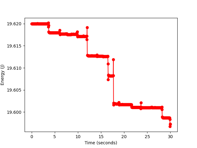
accuracy. The plot of
energy over time shows minimal change in the conservative system. A perfect integration scheme would
hold the energy constant.