Lyapunov Exponent Heatmap
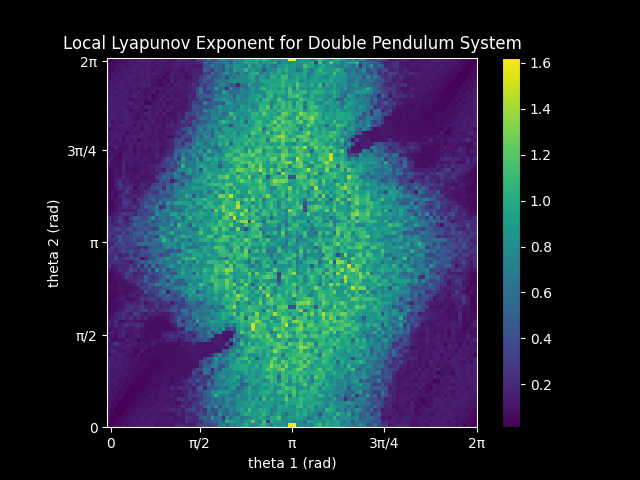
The grid represents a set of starting conditions for the double pendulum system where both masses start with no angular velocity. The x and y axis represent the initial angles for each of the rods in the system. \(\theta_1\) is the angle closer to the base. Note the symmetry in the system because any set of starting angles (\(\theta_1, \theta_2\)) have the same dynamics as (\(2π-\theta_1, 2π-\theta_2\)). Also note the streaks of low exponents moving in at a diagonal. These are the predictable dynamics centered around the periodic orbits where the two rods are in line with eachother.
The local Lyapunov exponent (\(\lambda)\) is a measure of how quickly neighboring starting conditions diverge given an initial condition \(x_0\). Therefore, it measures the local predictability of the system. The seperation vector between nearby initial conditions \(\delta \textbf{Z}(t)\) can be be described as growing at a rate: \[|\delta\textbf{Z}(t)| \approx e^{\lambda(t)}|\delta\textbf{Z}_0|\] For multidemensional systems there is a Lyaponov exponent associated with each direction (dimension) in the phase space. \[{\lambda_1, \lambda_2, ..., \lambda_n}\] Each Lyapunov exponent describes how each tangent vector encapsulated by the orthogonal matrix \(\textbf{Y}\) evolves from the initial uniform perturbation (\(\textbf{Y}_0\)) according to the rule: \[\dot{\textbf{Y}} = \textbf{J}\textbf{Y}\] Where \(\textbf{J}\) is the Jacobian matrix of the function at the point being evaluated. The matrix \(\textbf{Y}(t)\) describes how a small deviation from the initial conditions \(x_0\) evolve over time. The eigenvalues of the matrix represent the lyapunov exponent of the system after being averaged over the total integration time. They represent how much the initial perturbations are "stretched" in phase space. The eigendirections of the matrix represent the corresponding directions on which the state was stretched.
One way to efficiently approximate \(\lambda\) is to periodically normalize the matrix during the integration process in order to ensure the matrix represents only local perturbations. This can conveniently be done via the Gram-Shmidt process. Periodically, the \(\textbf{Y}\) matrix is factorized into an orthonormal \(\textbf{Q}\) matrix which represents the eigendirections of the local transformation. This is used as the uniform purturbation \(\textbf{Y}_1\) for the next cycle. The diagonal \(\textbf{R}\) matrix represents the Lyapunov exponents associated with each of these tangent vectors. The final singular Lyapunov exponent is given by the maximum of the average of these values for each calculation cycle. This is because local perturbations are stretched towards the dominant eigendirections, therefore the largest eigenvalue most accurately encapsulates the local dynamics.
For my calculations, I use a 4th order Runge—Kutta method for evaluating the dynamics of the initial conditions of interest. I let the \(\textbf{Y}\) matrix evolve according to the formula above for 1 second before re-factorizing. I then use the state of the true tragectory (which we want to perturbate) to calculate the new Jacobian. This 1 second cycle is repeated for 30 seconds after which the final value is calculated.